A Brief Tour of FLP Impossibility
One of the most important results in distributed systems theory was published in April 1985 by Fischer, Lynch and Patterson. Their short paper ‘Impossibility of Distributed Consensus with One Faulty Process’, which eventually won the Dijkstra award given to the most influential papers in distributed computing, definitively placed an upper bound on what it is possible to achieve with distributed processes in an asynchronous environment.
This particular result, known as the ‘FLP result’, settled a dispute that had been ongoing in distributed systems for the previous five to ten years. The problem of consensus - that is, getting a distributed network of processors to agree on a common value - was known to be solvable in a synchronous setting, where processes could proceed in simultaneous steps. In particular, the synchronous solution was resilient to faults, where processors crash and take no further part in the computation. Informally, synchronous models allow failures to be detected by waiting one entire step length for a reply from a processor, and presuming that it has crashed if no reply is received.
This kind of failure detection is impossible in an asynchronous setting, where there are no bounds on the amount of time a processor might take to complete its work and then respond with a message. Therefore it’s not possible to say whether a processor has crashed or is simply taking a long time to respond. The FLP result shows that in an asynchronous setting, where only one processor might crash, there is no distributed algorithm that solves the consensus problem.
In this post, I want to give a tour of the proof itself because, although it is quite subtle, it is short and profound. I’ll start by introducing consensus, and then after describing some notation and assumptions I’ll work through the main two lemmas in the paper.
If you want to follow along at home (highly, highly recommended) a copy of the paper is available here.
Consensus
The problem of consensus is genuinely fundamental to distributed systems research. Getting distributed processors to agree on a value has many, many applications. For example, the problem of deciding whether to commit a transaction to a database could be decided by a consensus algorithm between a majority of replicas. You can think of consensus as ‘voting’ for a value.
Several papers in the literature set the problem in the context of generals at different camps outside the enemy castle deciding whether or not to attack. A consensus algorithm that didn’t work would perhaps cause one general to attack while all the others stayed back - leaving the first general in trouble.
There are several variations on the consensus problem that differ in ‘strength’ - a solution to a stronger problem typically will solve weaker problems at the same time. A strong form of consensus is as follows:
Given a set of processors, each with an initial value:
- All non-faulty processes eventually decide on a value
- All processes that decide do so on the same value
- The value that has been decided must have proposed by some process
These three properties are referred to as termination, agreement and validity. Any algorithm that has these three properties can be said to solve the consensus problem.
Termination and agreement are fairly self explanatory - note that we explicitly do not require any particular behaviour from faulty nodes, which is just as well: they’re faulty! Validity is slightly more subtle, although it seems reasonable. The idea behind validity is that we want to exclude trivial solutions that just decide ‘No’ whatever the initial set of values is. Such an algorithm would satisfy termination and agreement, but would be completely vacuous, and no use to use at all.
The FLP proof actually concerns a slightly weaker form of consensus - for termination it is enough only that some non-faulty process decides. Note that it’s not enough to have one distinguished process that always decides its own value, as that process might fail, and another will have to take its place for even weak termination to be satisfied.
Clearly a solution to strong consensus will be a perfectly good solution for weak consensus as well, so by ruling out the possibility of the latter the FLP result similarly precludes a solution to the former.
For simplicity, the authors consider that the only values possible are 0 and 1. Every argument in the paper generalises to more values.
System Model
You can’t reasonably talk about a distributed algorithm without talking about the context it is designed to execute in and the assumptions it makes about the underlying distributed system. This set of assumptions is known as the system model and its choice has a profound effect on what algorithms are appropriate. Indeed, this paper is concerned entirely with an impossibility result on one particular class of system models.
There is a huge variety in system models, ranging from those based solidly on real-world experience to more theoretical models. Most share some basic properties in common: a network of distributed processors which are vertices in a connected graph where the edges are communication links along which messages may be sent. The variation comes in how each processor views the passage of time, whether links are reliable and how - if at all - processors are allowed to fail.
The FLP result is based on the asynchronous model, which is actually a class of models which exhibit certain properties of timing. The main characteristic of asynchronous models is that there is no upper bound on the amount of time processors may take to receive, process and respond to an incoming message. Therefore it is impossible to tell if a processor has failed, or is simply taking a long time to do its processing. The asynchronous model is a weak one, but not completely physically unrealistic. We have all encountered web servers that seem to take an arbitrarily long time to serve us a page. Now that mobile ad-hoc networks are becoming more and more pervasive, we see that devices in those networks may power down during processing to save battery, only to reappear later and continue as though nothing had happened. This introduces an arbitrary delay which fits the asynchronous model.
Other models are arguably more appropriate for networks like the Internet, but the asynchronous model is very general without being completely unrealistic.
The communication links between processors are assumed to be reliable. It was well known that given arbitrarily unreliable links no solution for consensus could be found even in a synchronous model; therefore by assuming reliable links and yet still proving consensus impossible in an asynchronous system the FLP result is made stronger. TCP gives reliable enough message delivery that this is a realistic assumption.
Processors are allowed to fail according to the fail-stop model - this simply means that processors that fail do so by ceasing to work correctly. There are more general failure models, such as Byzantine failures where processors fail by deviating arbitrarily from the algorithm they are executing. Again, by strengthening the model - by making strong assumptions about what is possible - the authors make their result much more general. The argument is as follows: if a given problem is proven unsolvable in a very restricted environment where only a few things can go wrong, it will certainly be unsolvable in an environment where yet more things can go wrong.
Formal Model
In order to formally model these properties, some notation needs to be introduced. In section 2 of the paper the system model is carefully defined. There are \(N>2\) processors which communicate by sending messages. A message is a pair \((p,m)\) where \(p\) is the processor the message is intended for, and \(m\) is the contents of the message. Messages are stored in an abstract data structure called the message buffer which is a multiset - simply a set where more than one of any element is allowed - which supports two operations. The first, send(p,m) simply places the message \((p,m)\) in the message buffer. The second, receive(p) either returns a message for processor \(p\) (and removes it from the message buffer) or the special value \(\theta\), which does nothing.
The semantics of receive aren’t completely intuitive (but make perfect sense!). If there are no messages in the message system addressed to \(p\) then receive(p) will return \(\theta\). However if there are messages for \(p\) then receive(p) will return one of them at random or \(\theta\). This captures the idea that messages may be delivered non-deterministically and that they may be received in any order, as well as being arbitrarily delayed as per the asynchronous model. The only requirement is that calling receive(p) infinitely many times will ensure that all messages in the message buffer are eventually delivered to \(p\). This means that messages may be arbitrarily delayed, but not completely lost.
A configuration is defined as the internal state of all of the processors - the current step in the algorithm that they are executing and the contents of their memory - together with the contents of the message buffer. The system moves from one configuration to the next by a step which consists of a processor \(p\) performing receive(p) and moving to another internal state. Therefore, the only way that the system state may evolve is by some processor receiving a message, or null, from the message buffer. Each step is therefore uniquely defined by the message that is received (possibly \(\theta\)) and the process that received it. That pair is called an event in the paper, so configurations move from one to another through events.
Since the receive operation is non-deterministic, there are many different possible executions for a given initial state (which for consensus is simply differentiated by the set of starting values that each processor has). In order to show that an algorithm solves consensus, we have to show that it satisfies validity, agreement and termination for every possible execution. The set of executions includes the possibility that processors are delayed arbitrarily, which we model by having them receive \(\theta\) for an arbitrary number of operations until they get their message. A particular execution, defined by a possibly infinite sequence of events from a starting configuration \(C\) is called a schedule and the sequence of steps taken to realise the schedule is a run.
Non-faulty processes take infinitely many steps in a run (presumably eventually just receiving \(\theta\) once the algorithm has finished its work) - otherwise a process is considered faulty. An admissible run is one where at most one process is faulty (capturing the failure requirements of the system model) and every message is eventually delivered (this means that every processor eventually gets chosen to receive infinitely many times). We say that a run is deciding provided that some process eventually decides according to the properties of consensus, and that a consensus protocol is totally correct if every admissible run is a deciding run.
With all those heavy definitions out of the way, the authors present their main theorem which is that no totally correct consensus algorithm exists. The idea behind it is to show that there is some admissible run - i.e. one with only one processor failure and eventual delivery of every message - that is not a deciding run - i.e. in which no processor eventually decides. This is enough to prove the general impossibility of consensus - it’s enough to show that there’s just one initial configuration in which a given protocol will not work because starting in that configuration can never be ruled out, and the result is a protocol which runs for ever (because no processor decides).
The Proof
As the paper says, ‘the basic idea is to show circumstances under which the protocol remains forever indecisive’. There are two steps to this, presented as two separate lemmas. The first demonstrates the existence of an initial condition which the second exploits. Things are tied together thereafter.
The First Lemma
(This is lemma 2 in the paper)
The point of the first lemma is to show that there is some initial configuration in which the decision is not predetermined, but in fact arrived as a result of the sequence of steps taken and the occurrence of any failure. For example, say that this initial configuration was two processors whose initial value was ‘0’ and one whose value was ‘1’. The authors show that what is decided from this configuration depends on the order in which messages are received and whether any of the processors fail, not just what the initial values of the processors are. This is due to the inherent non-determinism of the asynchronous system model.
The way this is done is quite neat. Suppose that the opposite was true - that all initial configurations have predetermined executions. There must be some initial configuration which results in a ‘0’ being decided and some for which ‘1’ is decided, by validity (which tells us that all results must be possible). Each configuration is uniquely determined by the set of initial values in the processors. We can order these values in a chain where two configurations are next to each other if they differ by only one value, so the only difference between two adjacent configurations is the starting value of one processor.
At some point along this chain, a ‘0’-deciding initial configuration must be next to a ‘1’-deciding one, and therefore they must differ by only one initial value. Call the ‘0’-deciding configuration \(C_0\) and the ‘1’-deciding configuration \(C_1\). Call the processor whose initial value is different in both \(p\). Now, from \(C_0\) there must be a run that decides ‘0’ even if \(p\) fails initially - because we allow one processor to fail. Therefore \(p\) neither sends nor receives any messages, so its initial value cannot be observed by the rest of the processors, one of whom must eventually decide ‘0’.
The crucial observation is that this run can also be made from \(C_1\). Because the configurations of \(C_0\) and \(C_1\) are exactly the same, except for the value at \(p\) which can’t contribute anything to the run because \(p\) has failed, any sequence of steps that \(C_0\) may take can also be taken by \(C_1\). But if they take exactly the same sequence of steps, then the eventual decision taken must be the same for both configurations. This contradicts our assumption that the result of the consensus algorithm is predetermined only by the initial configuration in \(C_0\) and \(C_1\), and that both configurations decide differently. So either one (or possibly both) of these configurations can potentially decide ‘0’ or ‘1’ and the eventual result depends on the pattern of failures and message deliveries.
We call the configurations that may lead to either decision value bivalent, and configurations that will only result in one value 0-valent or 1-valent. I’ll use these terms for the rest of this article.
The Second Lemma
(This is lemma 3 in the paper)
The second main lemma constitutes most of the body of the proof, although you wouldn’t know it to read it the first time. The statement of the lemma says, informally, that if a protocol starts from a bivalent configuration and there is a message \(e\) that is applicable to that configuration, then the set of configurations reachable through any sequence of messages where \(e\) is applied last contains a bivalent configuration.
Even more informally, but more intuitively, it says that if you delay a message that is pending any amount from one event to arbitrarily many, there will be one configuration in which you receive that message and end up in a bivalent state. This is crucial to the entire proof: you can probably see that guaranteeing that there is a path from a bivalent (where you see ‘bivalent’, read ‘undecided’ for clarity) configuration to another bivalent configuration by delaying a message long enough raises the possibility that an infinite loop will ensue and the protocol will remain forever undecided.
The proof of this lemma proceeds by contradiction. We need to set up some terminology as in the paper. Let \(C\) be a bivalent configuration and let \(e=(p,m)\) be some event that is applicable to \(C\). Let \(\mathbb{C}\) be the set of configurations reachable from \(C\) without applying \(e\), and let \(\mathbb{D}\) be the set of configurations resulting from applying \(e\) to configurations in \(\mathbb{C}\).
Assume that \(\mathbb{D}\) contains no bivalent configurations. The proof shows that this leads to a contradiction.
First, we show that \(\mathbb{D}\) contains both 0- and 1-valent configurations if it contains no bivalent configurations. Let \(E_i\) for \(i=0,1\) be an \(i\)-valent configuration reachable from \(C\). Both \(E_0\) and \(E_1\) exist because \(C\) is bivalent. For \(E_0\), if it is in \(\mathbb{C}\) (i.e. it has not received \(e\)) let \(F_0\) be the result of receiving \(e\) at \(E_0\). If it is not in \(\mathbb{C}\) then it has received \(e\); in this case let \(F_0\) be a configuration in \(\mathbb{D}\) from which \(E_0\) is reachable (i.e. the configuration that preceded \(E_0\) at the point that \(e\) was received).
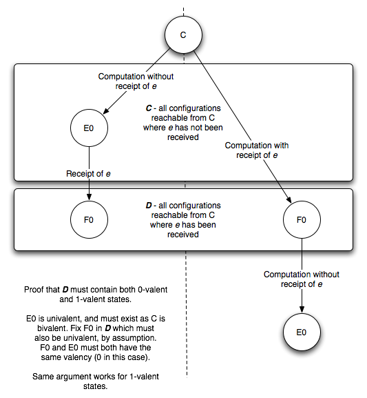
Figure 2.1
Figure 2.1: Proof that D must contain both 0- and 1-valent configurations if it contains no bivalent configuration
That confusing definition is quite a simple idea: we are fixing an \(F_0\) in \(\mathbb{D}\) that either comes before or after \(E_0\) depending on whether \(e\) was received in the run to \(E_0\).
Now we can see that \(F_0\) must be 0-valent. Either it comes before \(E_0\), in which case it too must be 0-valent, because it cannot be bivalent (by assumption) and if it were 1-valent the protocol would ‘change its mind’ between \(F_0\) and \(E_0\) which contradicts the definition of \(i\)-valent.
If \(F_0\) comes after \(E_0\), by the same argument it must be 0-valent. Therefore \(\mathbb{D}\) contains a 0-valent state.
We can define \(F_1\) relative to \(E_1\) similarly, to prove that \(\mathbb{D}\) contains a 1-valent configuration. Therefore we’ve shown that \(\mathbb{D}\) must contain both 0-valent and 1-valent configuration if it contains no bivalent configurations.
We use this fact to set up the rest of the lemma’s proof. By a similar argument to the ‘chain’ one used in the proof of the previous lemma, we can see that there must be two configurations \(C_0\) and \(C_1\) in \(\mathbb{C}\) where \(C_1\) is the result of receiving some message \(e\prime\) in \(C_0\), such that applying \(e\) to \(C_i\) gives an \(i\)-valent configuration. Call these configurations \(D_0\) and \(D_1\).
\(C_0\) and \(C_1\) are called ‘neighbours’ because they are separated by a single message delivery. Now, consider the message that separates them, \(e\prime=(p\prime,m\prime)\). Consider the two alternatives for the destination of \(e\prime\), that is \(p\prime\).
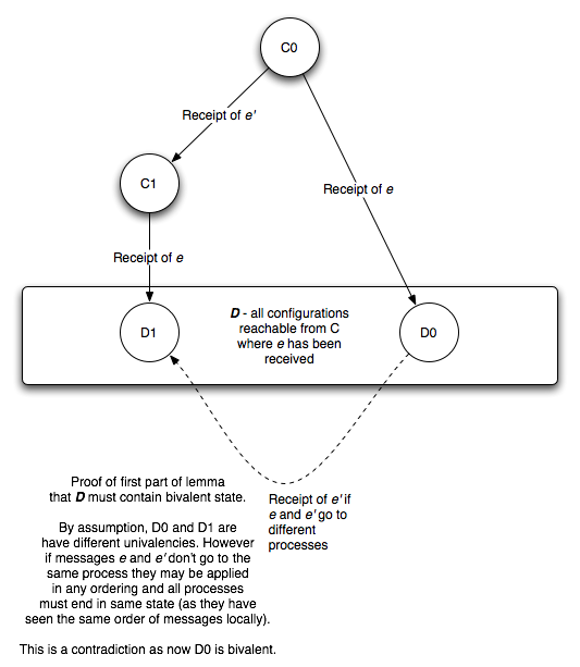
Figure2.2
Proof that D0 must be bivalent if the two states preceding D1 are separated by messages intended for different processes
-
If \(p\prime \neq p\) - i.e. the message that separates them is for a different processor than \(e\) - then we can get to \(D_1\) by receiving \(e\prime\) at \(D_0\). If the destination of a set of messages is different then we can receive them in any order to get to the same configuration, because all the processors see the same order of events, just at different times. (This is called the commutativity of schedules in the paper and is proved by its own lemma. I have left the proof out of this - already proof heavy - article). But \(D_0\) is 0-valent, and \(D_1\) is 1-valent. So we should not be able to reach \(D_1\) from \(D_0\), as again this would imply the protocol had changed its mind. Therefore this is a contradiction.
-
Instead consider \(p\prime = p\). Now consider a finite deciding run from \(C_0\) (the configuration such that receiving \(e\) results in a 0-valent configuration), in which \(p\) takes no steps (such a run must exist to cope with the possibility of \(p\) failing). Let \(A\) be the configuration that results at the end of that deciding run. We can also apply that run to either \(D_0\) or \(D_1\) to get two new configurations \(E_0\) and \(E_1\), and by the commutativity of schedules we can also receive \(e\) at \(A\) to get \(E_0\) (same set of messages, different delivery order), and \(e\prime\) followed by \(e\) at \(A\) to get \(E_1\). (Remember that \(e\) and \(e\prime\) are both available for receipt because \(p\) takes no steps in the deciding run). But this implies that \(A\) is bivalent, which is a contradiction since the run to \(A\) is deciding.
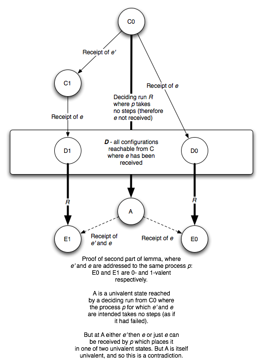
Figure 2.3
Proof that no deciding run from C0 exists if D contains only univalent configurations, and both messages preceding D1 are delivered to the same host
So, by contradiction, we have shown that \(\mathbb{D}\) must contain a bivalent configuration.
Bringing it all together
The final step is to show that any deciding run also allows the construction of an infinite non-deciding run. This is done by piecing together sections of runs in such a way as to avoid ever making a decision, that is to enter a univalent configuration.
Start from a bivalent initial configuration \(C_0\) (which exists as a result of the first lemma). To make the run admissible, place the processors in the system in a queue and have them receive messages in queue order, being placed at the back of the queue when they are done. This ensures that every message is eventually delivered.
Let \(e=(p,m)\) be the earliest message to the first processor in the queue; possibly a null message. Then by the second lemma we can reach a bivalent configuration \(C_1\) reachable from \(C_0\) where \(e\) is the last message received. Similarly, we can reach another bivalent configuration \(C_2\) from \(C_1\) by the same argument. And this may continue for ever. This run is admissible, but never reaches a decision, and it follows that the protocol is not totally correct.
Conclusion
Phew! That was a lot of technical proof to wade through. The meat of the proof is in the two lemmas. The first showed that there must be some initial configuration of the system in which the outcome of consensus is not already determined - you can’t just have a protocol that queries the state of the network and then indexes a massive look-up table, as failures or message delays are guaranteed to scupper that plan. This is the lemma where the possibility of failure is key: if there were no failures then the network state *would* be enough to determine consensus (because if there are no failures then message delay can be recognised for what it is).
The second lemma showed that, if you start in a bivalent configuration then it is always possible to reach another bivalent configuration by delaying a pending message. This can continue forever - even though all messages are eventually delivered - and so no protocol can guarantee that a univalent state might ever be reached.
What does this mean practically? The chance of entering that infinite undeciding loop can be made arbitrarily small - it’s one thing for nondecision to be possible, another thing entirely for it to be guaranteed. Still, there is much to be said for keeping this possibility in mind when your system livelocks during consensus and you don’t know why. Also, in practice, real systems aren’t always truly asynchronous.
This paper spawned a huge amount of subsequent work in the theoretical distributed systems community. Failure detectors were introduced by Toureg et. al. to characterise just how much the asynchronous model needed to be strengthened to allow for correct consensus. Randomised algorithms exist that practically make the probability of nondecision 0 if run for long enough. A lot of proofs by reduction were published that showed the equivalence of some problem to consensus, and therefore its impossibility. Different system models were postulated to circumvent the FLP problem, including partial synchrony which has had a lot of academic success.
The paper won the 2001 Dijkstra prize for the most influential paper in distributed computing. All three authors, Michael Fischer, Nancy Lynch and Mike Paterson are still very active and extremely eminent researchers in the field. Nancy Lynch, in particular, seems to have been involved in almost every important piece of work in distributed algorithms.